Reinforcement Learning
Introduction
Reinforcement learning is a framework for solving control tasks (also called decision problems) by building agents that learn from the environment by interacting with it through trial and error and receiving rewards (positive or negative) as unique feedback. It is a computational approach of learning from action. The idea behind Reinforcement Learning is that an agent (an AI) will learn from the environment by interacting with it (through trial and error) and receiving rewards (negative or positive) as feedback for performing actions.
Reinforcement Learning Framework
The RL Process
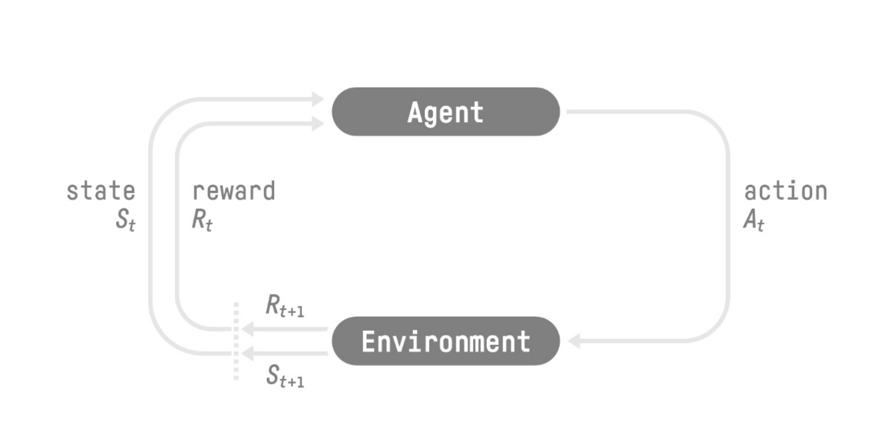
- Our Agent receives state $S_0$ from the Environment.
- Based on that state $S_0$ the Agent takes action $A_0$
- Environment goes to a new state $S_1$ .
- The environment gives some reward $R_1$ to the Agent (Positive Reward +1).
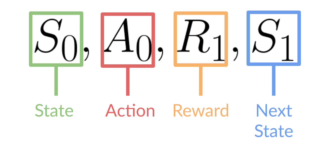
RL process is a loop that outputs a sequence of state, action, reward and next state.
Markov Property
RL process is also called the Markov Decision Process (MDP). The Markov Property implies that our agent needs only the current state to decide what action to take and not the history of all the states and actions they took before.
The reward hypothesis
The goal of any RL agent is to maximize its expected cumulative reward (also called expected return). The central idea of Reinforcement Learning is the reward hypothesis: all goals can be described as the maximization of the expected return (expected cumulative reward). That’s why in Reinforcement Learning, to have the best behavior, we aim to learn to take actions that maximize the expected cumulative reward.
Observations/States Space
Observations/States are the information our agent gets from the environment.
- State s : is a complete description of the state of the world (there is no hidden information). eg. In chess game, we receive a state from the environment since we have access to the whole check board information.
- Observation o: is a partial description of the state in a partially observed environment. e.g. In Super Mario Bros, we only see a part of the level close to the player, so we receive an observation.
Action Space
The Action space is the set of all possible actions in an environment.
- Discrete space: the number of possible actions is finite. e.g. Super Mario Bros, we have only 5 possible actions: 4 directions and jumping.
- Continuous space: the number of possible actions is infinite. e.g. Self Driving Car agent has an infinite number of possible actions.
Discounted Rewards
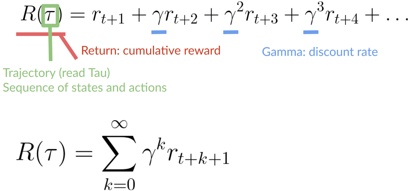
The reward is fundamental in RL because it’s the only feedback for the agent. However, in reality, we can’t just add them. To calculate the expected cumulative reward (expected return), we discount the rewards: the rewards that come sooner (at the beginning of the game) are more probable to happen since they are more predictable than the long term future reward.
To discount the rewards:
- We define a discount rate called gamma (between 0 and 1). Most of the time between 0.99 and 0.95.
- The larger the gamma, the smaller the discount. This means our agent cares more about the long-term reward.
- On the other hand, the smaller the gamma, the bigger the discount. This means our agent cares more about the short term reward.
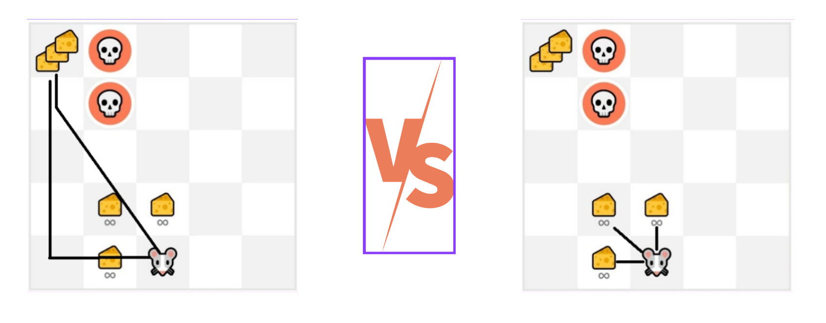
2. Then, each reward will be discounted by gamma to the exponent of the time step. As the time step increases, the cat gets closer to us, so the future reward is less and less likely to happen.
Type of Tasks
A task is an instance of a Reinforcement Learning problem. We can have two types of tasks: episodic and continuing.
Episodic Task
In this case, we have a starting point and an ending point (a terminal state). This creates an episode: a list of States, Actions, Rewards, and new States. e.g. In Super Mario Bros, episode begin at the launch of a new Mario Level and ending when you’re killed or you reached the end of the level
Continuing Tasks
These are tasks that continue forever (no terminal state). In this case, the agent must learn how to choose the best actions and simultaneously interact with the environment. For instance, an agent that does automated stock trading. For this task, there is no starting point and terminal state. The agent keeps running until we decide to stop it.
Exploration/Exploitation Trade-off
- Exploration is exploring the environment by trying random actions in order to find more information about the environment.
- Exploitation is exploiting known information to maximize the reward.
We need to balance how much we explore the environment and how much we exploit what we know about the environment.
The Policy π: the Agent’s Brain

Approaches for solving RL problems
How to build an RL agent that can select the actions that maximize its expected cumulative reward?
There are two approaches to train our agent to find this optimal policy π*:
- Directly, by teaching the agent to learn which action to take, given the current state: Policy-Based Methods.
- Indirectly, teach the agent to learn which state is more valuable and then take the action that leads to the more valuable states: Value-Based Methods.
Policy-Based Methods
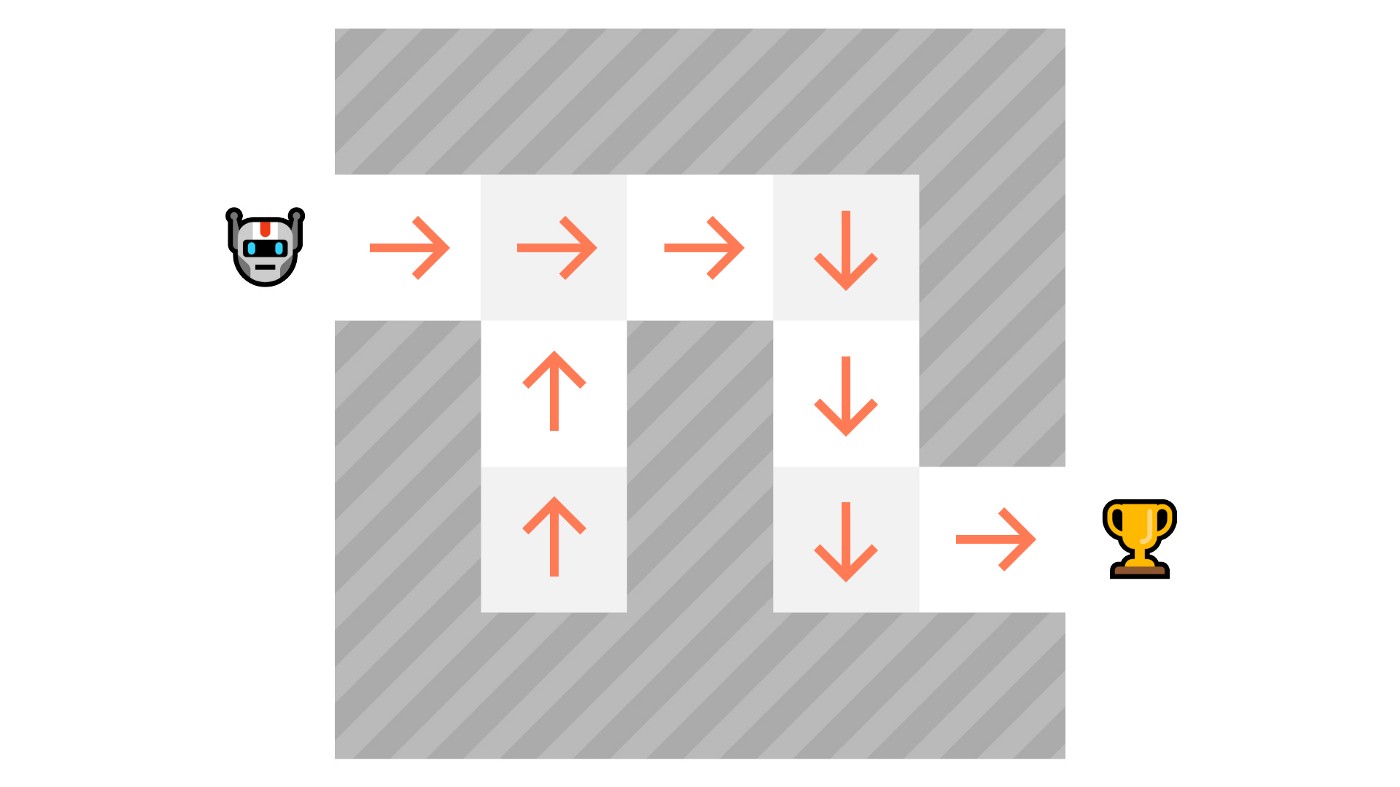
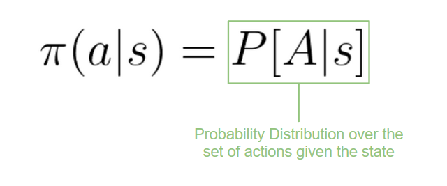
In Policy-Based methods, we learn a policy function directly. This function will define a mapping between each state and the best corresponding action. We can also say that it’ll define a probability distribution over the set of possible actions at that state.
We have two types of policies:
Deterministic Policy
A policy at a given state will always return the same action.

Stochastic Policy
Outputs a probability distribution over actions.
Value-based methods
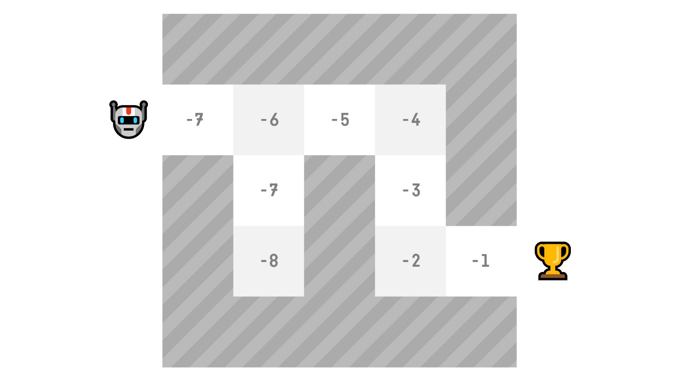
Here, will select the state with the biggest value defined by the value function: -7, then -6, then -5 (and so on) to attain the goal.
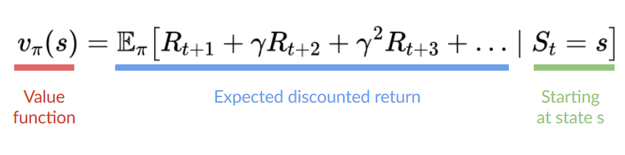
In value-based methods, instead of training a policy function, we train a value function that maps a state to the expected value of being at that state.
The value of a state is the expected discounted return the agent can get if it starts in that state, and then act according to our policy. “Act according to our policy” just means that our policy is “going to the state with the highest value”.
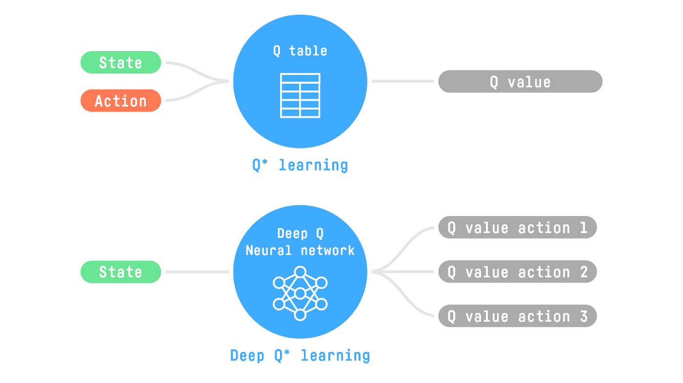
The “Deep” in Reinforcement Learning
References
[1]. Introduction to Deep Reinforcement Learning - Hugging Face Course. (n.d.). https://huggingface.co/deep-rl-course/unit1/introduction?fw=pt